Factor Analysis of Segregation Measures: A Replication
While reading A Wealth and Status-Based Model of Residential Segregation, I noticed its discussion of Massey and Denton (1988), who reviewed 20 segregation indices and applied them to 1980 census data from 60 metropolitan statistical areas (MSAs). Using factor analysis, Massey and Denton classified these indices into five underlying dimensions: evenness, exposure, clustering, centralization, and concentration.
However, they appear to have chosen five factors a priori, based on their review of the literature, rather than using the data to determine how many factors to retain. So, I decided to replicate their analysis using parallel analysis to determine the number of factors empirically.
I also broadened the analysis in two ways. Instead of restricting the sample to 60 MSAs, I used every contemporary metropolitan area with at least 1,000 members of the focal racial group and at least 1,000 non-Hispanic White-alone residents1. And instead of examining only 1980, I repeated the analysis for 1990, 2000, 2010, and 2020 to see how stable the findings are over four decades. The national-sample result is remarkably consistent: parallel analysis retains three factors in every census year. The fixed panel corresponding to the original 60 metropolitan identities produces a more conservative result, as discussed below.
Massey and Denton’s five dimensions describe the different ways in which residential segregation might occur:
- Evenness: How evenly distributed is a group across residential areas?
- Exposure: How much potential contact do members of one group have with members of another group?
- Concentration: How much physical space does a group occupy?
- Centralization: How concentrated is a group in the city center?
- Clustering: To what degree does a group disproportionately live in contiguous areas?
How many factors are there?
The national sample consistently yields three factors, not five.
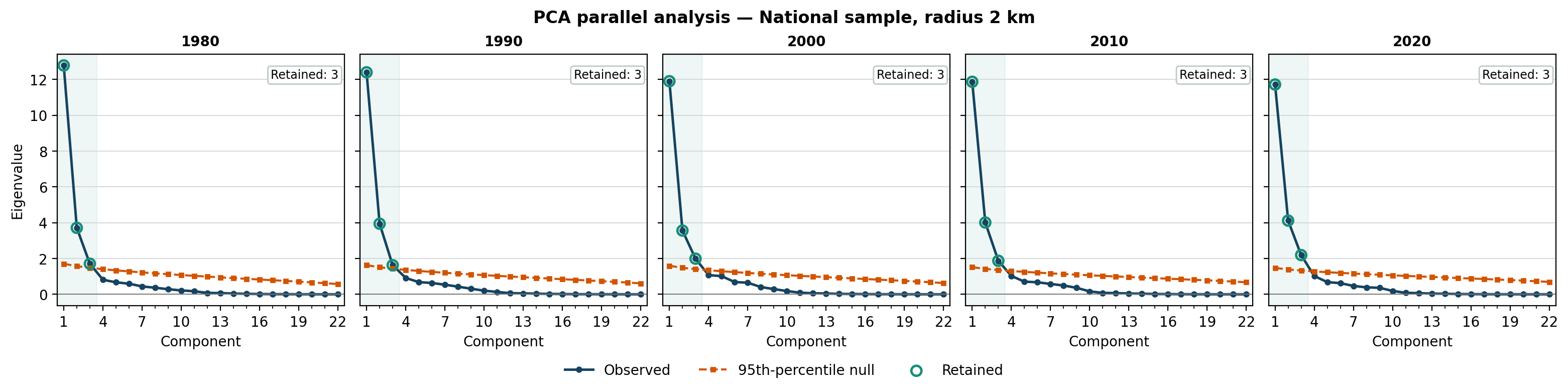
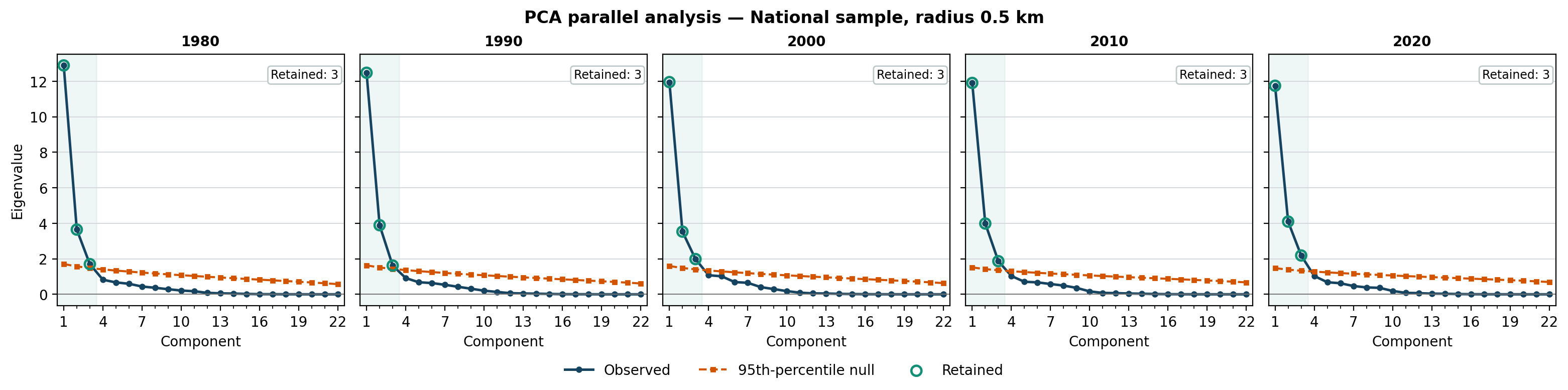
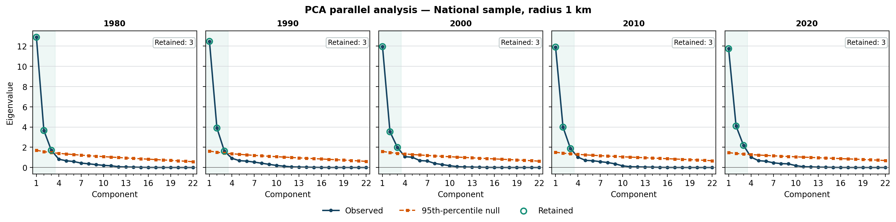
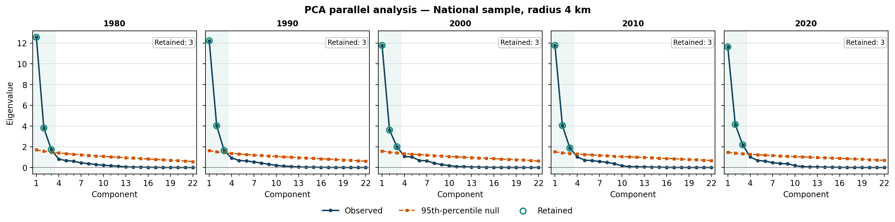
I’ve shown the findings for when the local-environment radius for the spatial measures is set at 2km, but the same result happens when we use 0.5, 1, or 4 km (see the Appendix).
Does the result depend on the sample?
As a robustness check, I repeated the analysis using a fixed panel corresponding to Massey and Denton’s original 60 metropolitan identities, following the same metro names while using each census year’s contemporary boundaries. The number of retained factors is the same at every spatial radius within a given sample and year:
| Sample | 1980 | 1990 | 2000 | 2010 | 2020 |
|---|---|---|---|---|---|
| National sample | 3 | 3 | 3 | 3 | 3 |
| Original-metro panel | 2 | 2 | 2 | 2 | 3 |
The fixed panel has a much smaller weighted effective sample size (between 69 and 92 observations, compared with 230 to 472 in the national sample) so parallel analysis is more conservative. Still, we can see that the data does not support five factors.
What do the factors measure?
The three factors are Evenness, Isolation, and Concentration. Expand each factor below for its interpretation and loadings.
Evenness
This is pretty similar to the original Evenness dimension that Massey and Denton found; it measures how evenly distributed the minority and majority groups are.
Factor loadings
| Index | 1980 | 1990 | 2000 | 2010 | 2020 |
|---|---|---|---|---|---|
| Atkinson, $b = 0.5$ | 1.00 | 0.99 | 0.99 | 1.00 | 0.99 |
| Atkinson, $b = 0.9$ | 1.00 | 0.98 | 0.99 | 1.00 | 0.99 |
| Information theory ($H$) | 0.99 | 0.99 | 0.97 | 1.00 | 0.99 |
| Spatial information theory ($H_s$) | 0.98 | 0.99 | 0.96 | 1.00 | 1.00 |
| Spatial dissimilarity ($D_s$) | 0.96 | 0.97 | 0.99 | 0.99 | 0.99 |
| Gini ($G$) | 0.98 | 0.97 | 0.98 | 0.98 | 0.98 |
| Dissimilarity ($D$) | 0.96 | 0.97 | 0.99 | 0.98 | 0.99 |
| Atkinson, $b = 0.1$ | 0.88 | 0.93 | 0.96 | 0.96 | 0.96 |
| Correlation ratio ($\eta^2$) | 0.94 | 0.95 | 0.90 | 0.94 | 0.94 |
| Spatial proximity ($\mathrm{SP}$) | 0.82 | 0.92 | 0.90 | 0.93 | 0.91 |
| Divergence index ($\mathrm{DIV}$) | 0.81 | 0.81 | 0.77 | 0.85 | 0.86 |
| Relative clustering ($\mathrm{RCL}$) | 0.60 | 0.69 | 0.72 | 0.59 | 0.55 |
| Relative centralization ($\mathrm{RCE}$) | 0.22 | 0.46 | 0.64 | 0.45 | 0.46 |
Isolation
Broadly speaking, these indices measure how much contact a random member of the focal group is expected to have with other members of the same group.
Factor loadings
| Index | 1980 | 1990 | 2000 | 2010 | 2020 |
|---|---|---|---|---|---|
| Distance-decay isolation ($\mathrm{DP}_{xx}$) | 0.98 | 0.97 | 0.98 | 0.95 | 0.96 |
| Spatial isolation (${}_xP_x^{(s)}$) | 0.89 | 0.90 | 0.94 | 0.92 | 0.93 |
| Isolation (${}_xP_x$) | 0.85 | 0.87 | 0.93 | 0.91 | 0.93 |
| Absolute concentration ($\mathrm{ACO}$) | -0.83 | -0.87 | -0.31 | -0.90 | -0.92 |
Concentration
This combines indices that measure how concentrated a group is in the city center with indices that measure how concentrated a group is in general.
Factor loadings
| Index | 1980 | 1990 | 2000 | 2010 | 2020 |
|---|---|---|---|---|---|
| Absolute centralization ($\mathrm{ACE}$) | 0.84 | 0.87 | 0.62 | 0.90 | 0.90 |
| Delta ($\mathrm{DEL}$) | 0.84 | 0.82 | 0.68 | 0.83 | 0.86 |
| Proportion central city ($\mathrm{PCC}$) | 0.82 | 0.83 | 0.61 | 0.77 | 0.77 |
| Relative concentration ($\mathrm{RCO}$) | 0.82 | 0.74 | 0.92 | 0.50 | 0.55 |
| Relative centralization ($\mathrm{RCE}$) | 0.69 | 0.46 | 0.28 | 0.40 | 0.39 |
Why are there fewer than five factors?
So, are there really only three dimensions of segregation? The national sample says three, while the fixed panel generally says two. But neither supports five. I’d argue that there are three relevant dimensions, even if the smaller fixed panel does not always distinguish all three empirically.
A problem that immediately jumped out at me when reading about the five dimensions was that the Centralization dimension makes an assumption not about how a group is distributed, but about where the group is distributed. This assumption makes me uneasy. I don’t like my mathematical measures to bake in such messy, empirical assumptions. Now, it does make sense that, given the fact that minority groups tend to be located near the center of urban areas, we’d expect centralization to be correlated with concentration. But I’d prefer to use concentration measures and then, once we determine that certain groups tend to end up concentrated, ask where those groups are concentrated. If that turns out to be the city center, then great.
What about the two dimensions that don’t show up in my factor analysis, Exposure and Clustering? Well, conceptually, clustering seems related to evenness: if a group is all clustered together, then it isn’t evenly distributed. As for exposure, that seems related to isolation. If a group is isolated, that is, its members are particularly likely to live near one another, then they’re not very exposed to members of other groups.
So, it doesn’t actually seem like we needed five dimensions in the first place.
Which measures should we use?
Which measures should be used for each factor? For the Evenness factor, there are seven indices with consistently near-perfect loadings, so really, we could choose any of them and we’d be fine. But the dissimilarity index ($D$) seems to be the most popular, so we’ll go with that.
For the Isolation factor, the three highest-loading indices are, well, isolation indices. Of these three, distance-decay isolation and spatial isolation seem the most conceptually appropriate: we should expect neighboring tracts to matter when determining isolation. Of these, distance-decay isolation consistently loads higher, so let’s go with that.
For the Concentration factor, I’d prefer to avoid any measures that explicitly refer to or rely on the idea of a city center, which leaves delta ($\text{DEL}$) as our best option.
So, if you want to measure segregation, I would distinguish three dimensions: evenness, isolation, and concentration. If you’re interested in evenness, use the dissimilarity index. If you’re interested in isolation, use distance-decay isolation. If you’re interested in concentration, use the delta index.
Appendix
Measures of Segregation
The analysis uses 22 nonredundant indices: 18 from the original Massey-Denton battery and four later extensions. Expand any measure below for its interpretation and formula.
Population and area notation:
- $x_i$ and $y_i$ are the focal-group and non-Hispanic-White populations of tract $i$.
- $t_i=x_i+y_i$ is the tract’s two-group population.
- $X$, $Y$, and $T$ are the corresponding metropolitan totals.
- $p_i=x_i/t_i$ is the focal-group share of tract $i$, and $P=X/T$ is the focal-group share of the metropolitan population.
- $a_i$ is tract land area (in square miles).
For the original proximity measures:
- $d_{ij}$ is the distance in miles between the representative points of tracts $i$ and $j$.
- $z_{ij}=e^{-d_{ij}}$ is the distance-decay weight.
- Within a tract, self-distance is approximated as $d_{ii}=\sqrt{0.6\,a_i}$. This is to avoid treating every resident of a tract as if they’re in the exact same place.
For the added local-environment measures:
- $r_{ij}$ is the distance in kilometers between tracts $i$ and $j$.
- $h$ is the local-environment radius.
Nearby tracts are weighted using the biweight kernel:
\[w_{ij}(h)= \begin{cases} [1-(r_{ij}/h)^2]^2, & r_{ij}<h,\\ 0, & r_{ij}\ge h. \end{cases}\]The resulting focal-group share of tract $i$’s local environment is:
\[q_i=\frac{\sum_j w_{ij}(h)x_j}{\sum_j w_{ij}(h)t_j}.\]Indices of Segregation
Dissimilarity ($D$)
Massey and Denton (1988) dimension: Evenness
Dissimilarity is the share of either group that would have to move to a different tract for every tract to have the same two-group composition as the metropolitan area. It ranges from zero under identical tract distributions to one under complete separation.
\[D=\frac{1}{2}\sum_i\left|\frac{x_i}{X}-\frac{y_i}{Y}\right|\]Formula sources: Massey and Denton (1988) and U.S. Census Bureau, Housing Patterns: Appendix B.
Gini ($G$)
Massey and Denton (1988) dimension: Evenness
The segregation Gini compares the focal-group proportions of every pair of tracts, weighting pairs by their two-group populations. Like dissimilarity, it is zero when tract compositions are identical and one under complete separation, but it uses the entire segregation curve rather than a single cutoff.
\[G=\frac{\sum_i\sum_j t_i t_j|p_i-p_j|}{2T^2P(1-P)}\]Formula sources: Massey and Denton (1988) and U.S. Census Bureau, Housing Patterns: Appendix B.
Information Theory ($H$)
Massey and Denton (1988) dimension: Evenness
Information theory measures the proportional reduction in racial/ethnic entropy obtained by knowing a person’s tract. It is zero when every tract reproduces the metropolitan composition and approaches one as tracts become internally homogeneous.
Writing $E(q)=-q\log q-(1-q)\log(1-q)$,
\[H=1-\frac{\sum_i t_iE(p_i)}{TE(P)}\]Formula sources: Massey and Denton (1988) and U.S. Census Bureau, Housing Patterns: Appendix B.
Atkinson, $b = 0.1$
Massey and Denton (1988) dimension: Evenness
This is the low-parameter member of the Atkinson segregation family. The parameter changes which parts of the tract-composition distribution receive the most weight; using several values tests whether the result depends on that normative weighting. Higher values indicate greater unevenness.
\[A_b=1-\frac{P}{1-P}\left[\frac{\sum_i t_i p_i^b(1-p_i)^{1-b}}{PT}\right]^{1/(1-b)},\qquad b=0.1\]Formula sources: Massey and Denton (1988) and U.S. Census Bureau, Housing Patterns: Appendix B.
Atkinson, $b = 0.5$
Massey and Denton (1988) dimension: Evenness
This is the midpoint specification of the Atkinson index. It gives a comparatively balanced weighting to focal- and reference-group representation across tracts. Higher values indicate greater unevenness.
\[A_b=1-\frac{P}{1-P}\left[\frac{\sum_i t_i p_i^b(1-p_i)^{1-b}}{PT}\right]^{1/(1-b)},\qquad b=0.5\]Formula sources: Massey and Denton (1988) and U.S. Census Bureau, Housing Patterns: Appendix B.
Atkinson, $b = 0.9$
Massey and Denton (1988) dimension: Evenness
This is the high-parameter member of the Atkinson segregation family. Together with the 0.1 and 0.5 versions, it checks the sensitivity of measured unevenness to the Atkinson weighting parameter. Higher values indicate greater unevenness.
\[A_b=1-\frac{P}{1-P}\left[\frac{\sum_i t_i p_i^b(1-p_i)^{1-b}}{PT}\right]^{1/(1-b)},\qquad b=0.9\]Formula sources: Massey and Denton (1988) and U.S. Census Bureau, Housing Patterns: Appendix B.
Divergence Index ($\mathrm{DIV}$)
Massey and Denton (1988) dimension: Not included in their review
The divergence index is the population-weighted Kullback-Leibler divergence between each tract’s two-group composition and the metropolitan composition. It is zero when all tracts match the metropolitan area and increases as their compositions diverge. Unlike many normalized indices, it is not constrained to a zero-to-one scale.
\[\mathrm{DIV}=\sum_i\frac{t_i}{T}\left[p_i\log\frac{p_i}{P}+(1-p_i)\log\frac{1-p_i}{1-P}\right]\]Formula source: Roberto (2015), The Divergence Index.
Spatial Information Theory ($H_s$)
Massey and Denton (1988) dimension: Not included in their review
This replaces each tract’s composition in the information-theory index with the composition of its kernel-weighted local environment.
If $q_i$ is the focal-group proportion in tract $i$’s local environment,
\[H_s=1-\frac{\sum_i t_iE(q_i)}{TE(P)}\]Formula framework: Reardon and O’Sullivan (2004), Measures of Spatial Segregation. The displayed equation is the tract-centroid, biweight-kernel implementation used in this analysis.
Spatial Dissimilarity ($D_s$)
Massey and Denton (1988) dimension: Not included in their review
Spatial dissimilarity ($D_s$) measures the population-weighted absolute difference between each tract’s local-environment composition and the metropolitan composition.
\[D_s=\frac{\sum_i t_i|q_i-P|}{2TP(1-P)}\]Formula framework: Reardon and O’Sullivan (2004), Measures of Spatial Segregation. The displayed equation is the tract-centroid, biweight-kernel implementation used in this analysis.
Isolation (${}_xP_x$)
Massey and Denton (1988) dimension: Exposure
Isolation is the expected focal-group share of the tract occupied by a randomly selected focal-group member. It therefore combines segregation with the focal group’s overall metropolitan prevalence: even under equal tract composition, its baseline is $P$ rather than zero.
\[xP_x=\sum_i\frac{x_i}{X}p_i\]Formula sources: Massey and Denton (1988) and U.S. Census Bureau, Housing Patterns: Appendix B.
Correlation Ratio ($\eta^2$)
Massey and Denton (1988) dimension: Exposure
The correlation ratio rescales isolation relative to the focal group’s metropolitan share. It can be interpreted as the proportion of variance in individual group membership associated with tract membership: zero indicates no tract differentiation and one indicates complete separation.
\[\eta^2=\frac{xP_x-P}{1-P}\]Formula sources: Massey and Denton (1988) and U.S. Census Bureau, Housing Patterns: Appendix B.
Distance-Decay Isolation ($\mathrm{DP}_{xx}$)
Massey and Denton (1988) dimension: Clustering
Distance-decay isolation replaces same-tract contact with potential contact across all tract pairs. Pairwise influence declines exponentially with distance, while a tract’s self-distance is approximated from its area. Higher values mean that the average focal-group resident’s spatial surroundings contain a larger focal-group share.
\[\mathrm{DP}_{xx}=\sum_i\frac{x_i}{X}\left(\frac{\sum_j z_{ij}x_j}{\sum_j z_{ij}t_j}\right)\]Formula sources: Massey and Denton (1988) and U.S. Census Bureau, Housing Patterns: Appendix B.
Spatial Isolation (${}_xP_x^{(s)}$)
Massey and Denton (1988) dimension: Not included in their review
Spatial isolation (${}_xP_x^{(s)}$) is the expected focal-group proportion in the kernel-weighted local environment of a randomly selected focal-group resident. Unlike distance-decay isolation, its influence has a finite outer radius and follows a biweight kernel.
\[xP_x^{(s)}=\sum_i\frac{x_i}{X}q_i\]Formula framework: Reardon and O’Sullivan (2004), Measures of Spatial Segregation. The displayed equation is the tract-centroid, biweight-kernel implementation used in this analysis.
Delta ($\mathrm{DEL}$)
Massey and Denton (1988) dimension: Concentration
Delta compares the focal group’s distribution across tracts with the distribution of metropolitan land area. It is the share of the focal population that would have to relocate for its tract distribution to match the distribution of land area.
If $a_i$ is tract land area and $A=\sum_i a_i$,
\[\mathrm{DEL}=\frac{1}{2}\sum_i\left|\frac{x_i}{X}-\frac{a_i}{A}\right|\]Formula sources: Massey and Denton (1988) and U.S. Census Bureau, Housing Patterns: Appendix B.
Absolute Concentration ($\mathrm{ACO}$)
Massey and Denton (1988) dimension: Concentration
Absolute concentration compares the average tract area occupied by focal-group members with the smallest and largest areas that could contain the same population under the observed tract structure. Let $\bar a_x=\sum_i x_i a_i/X$. Let $\bar a_{\min}$ and $\bar a_{\max}$ be the population-weighted mean areas obtained by filling the smallest and largest tracts respectively until the accumulated two-group population reaches $X$. Then
\[\mathrm{ACO}=1-\frac{\bar a_x-\bar a_{\min}}{\bar a_{\max}-\bar a_{\min}}.\]Higher values indicate that the focal group occupies relatively little physical space. The published normalization can leave its nominal range in unusual metros where the designated focal group is overwhelmingly dominant; those values were retained rather than clipped.
Formula sources: Massey and Denton (1988) and U.S. Census Bureau, Housing Patterns: Appendix B.
Relative Concentration ($\mathrm{RCO}$)
Massey and Denton (1988) dimension: Concentration
Relative concentration compares the focal group’s population-weighted mean tract area with that of the reference group, normalized by the metropolitan area’s feasible area limits. With $\bar a_x=\sum_i x_i a_i/X$, $\bar a_y=\sum_i y_i a_i/Y$, and the same $\bar a_{\min}$ and $\bar a_{\max}$ used for $\mathrm{ACO}$,
\[\mathrm{RCO}=\frac{\bar a_x/\bar a_y-1}{\bar a_{\min}/\bar a_{\max}-1}.\]Positive values indicate that the focal group occupies less space than the reference group; negative values indicate the reverse.
Formula sources: Massey and Denton (1988) and U.S. Census Bureau, Housing Patterns: Appendix B.
Proportion Central City ($\mathrm{PCC}$)
Massey and Denton (1988) dimension: Centralization
$\mathrm{PCC}$ is simply the proportion of the focal metropolitan population living within the year’s official central or principal city boundaries. When a metropolitan area has multiple official central/principal cities, all of them count.
\[\mathrm{PCC}=\frac{\sum_{i\in\text{central city}}x_i}{X}\]Formula sources: Massey and Denton (1988) and U.S. Census Bureau, Housing Patterns: Appendix B.
Absolute Centralization ($\mathrm{ACE}$)
Massey and Denton (1988) dimension: Centralization
After ordering tracts from nearest to farthest from the metropolitan center, define $C_i^x=\sum_{j\le i}x_j/X$ and $C_i^a=\sum_{j\le i}a_j/\sum_j a_j$. Absolute centralization is
\[\mathrm{ACE}=\sum_{i=1}^{n-1}\left(C_i^xC_{i+1}^a-C_{i+1}^xC_i^a\right).\]Positive values indicate centralization, zero indicates no systematic central tendency, and negative values indicate decentralization toward the periphery.
Formula sources: Massey and Denton (1988) and U.S. Census Bureau, Housing Patterns: Appendix B.
Relative Centralization ($\mathrm{RCE}$)
Massey and Denton (1988) dimension: Centralization
After ordering tracts from nearest to farthest from the center, define $C_i^x=\sum_{j\le i}x_j/X$ and $C_i^y=\sum_{j\le i}y_j/Y$. Relative centralization is
\[\mathrm{RCE}=\sum_{i=1}^{n-1}\left(C_i^xC_{i+1}^y-C_{i+1}^xC_i^y\right).\]Positive values mean the focal group is more centralized than non-Hispanic White residents; negative values mean it is less centralized.
Formula sources: Massey and Denton (1988) and U.S. Census Bureau, Housing Patterns: Appendix B.
Absolute Clustering ($\mathrm{ACL}$)
Massey and Denton (1988) dimension: Clustering
Absolute clustering compares the distance-weighted proximity of focal-group residents to one another with the proximity expected under a uniform spatial distribution, normalized by the proximity of the total two-group population. Define
\[C_x=\sum_i\frac{x_i}{X}\sum_jz_{ij}x_j,\qquad C_t=\sum_i\frac{x_i}{X}\sum_jz_{ij}t_j,\qquad U=\frac{X}{n^2}\sum_i\sum_jz_{ij}.\]Then
\[\mathrm{ACL}=\frac{C_x-U}{C_t-U}.\]Higher values indicate a more tightly clustered focal population.
Formula sources: Massey and Denton (1988) and U.S. Census Bureau, Housing Patterns: Appendix B.
Spatial Proximity ($\mathrm{SP}$)
Massey and Denton (1988) dimension: Clustering
Define focal-group, reference-group, and total-population proximity as
\[P_{xx}=\frac{\sum_i\sum_jx_ix_jz_{ij}}{X^2},\qquad P_{yy}=\frac{\sum_i\sum_jy_iy_jz_{ij}}{Y^2},\qquad P_{tt}=\frac{\sum_i\sum_jt_it_jz_{ij}}{T^2}.\]Spatial proximity is
\[\mathrm{SP}=\frac{XP_{xx}+YP_{yy}}{TP_{tt}}.\]A value of one indicates no excess same-group proximity; values above one indicate that members of the two groups tend to live nearer members of their own group.
Formula sources: Massey and Denton (1988) and U.S. Census Bureau, Housing Patterns: Appendix B.
Relative Clustering ($\mathrm{RCL}$)
Massey and Denton (1988) dimension: Clustering
Using $P_{xx}$ and $P_{yy}$ as defined for $\mathrm{SP}$, relative clustering is
\[\mathrm{RCL}=\frac{P_{xx}}{P_{yy}}-1.\]Zero means equal clustering, positive values mean the focal group is more clustered, and negative values mean the reference group is more clustered.
Formula sources: Massey and Denton (1988) and U.S. Census Bureau, Housing Patterns: Appendix B.
Parallel Analysis for Other Distances
Factor Loadings at Other Distances
The factors are matched and sign-aligned to each radius’s 1980 solution. As in the primary 2-km analysis, each table includes only indices whose mean absolute loading on that factor across the five censuses is at least .40, ordered by that mean.
0.5-km radius
Factor 1: Evenness
| Index | 1980 | 1990 | 2000 | 2010 | 2020 |
|---|---|---|---|---|---|
| Atkinson, $b = 0.5$ | 1.01 | 0.99 | 0.99 | 1.00 | 1.00 |
| Atkinson, $b = 0.9$ | 1.00 | 0.98 | 0.99 | 1.00 | 1.00 |
| Spatial information theory ($H_s$) | 0.99 | 0.99 | 0.97 | 1.00 | 1.00 |
| Information theory ($H$) | 0.99 | 0.99 | 0.97 | 1.00 | 1.00 |
| Gini ($G$) | 0.98 | 0.97 | 0.99 | 0.98 | 0.98 |
| Dissimilarity ($D$) | 0.96 | 0.97 | 0.99 | 0.98 | 0.99 |
| Spatial dissimilarity ($D_s$) | 0.96 | 0.97 | 0.99 | 0.98 | 0.99 |
| Atkinson, $b = 0.1$ | 0.89 | 0.93 | 0.96 | 0.97 | 0.96 |
| Correlation ratio ($\eta^2$) | 0.94 | 0.95 | 0.90 | 0.94 | 0.94 |
| Spatial proximity ($\mathrm{SP}$) | 0.82 | 0.92 | 0.90 | 0.93 | 0.91 |
| Divergence index ($\mathrm{DIV}$) | 0.81 | 0.81 | 0.77 | 0.85 | 0.87 |
| Relative clustering ($\mathrm{RCL}$) | 0.60 | 0.69 | 0.72 | 0.59 | 0.55 |
| Relative centralization ($\mathrm{RCE}$) | 0.22 | 0.46 | 0.64 | 0.45 | 0.46 |
Factor 2: Isolation
| Index | 1980 | 1990 | 2000 | 2010 | 2020 |
|---|---|---|---|---|---|
| Distance-decay isolation ($\mathrm{DP}_{xx}$) | 0.99 | 0.97 | 0.98 | 0.95 | 0.96 |
| Spatial isolation (${}_xP_x^{(s)}$) | 0.85 | 0.88 | 0.93 | 0.91 | 0.92 |
| Isolation (${}_xP_x$) | 0.85 | 0.88 | 0.93 | 0.91 | 0.92 |
| Absolute concentration ($\mathrm{ACO}$) | -0.83 | -0.87 | -0.30 | -0.90 | -0.92 |
Factor 3: Concentration
| Index | 1980 | 1990 | 2000 | 2010 | 2020 |
|---|---|---|---|---|---|
| Absolute centralization ($\mathrm{ACE}$) | 0.85 | 0.87 | 0.62 | 0.90 | 0.90 |
| Delta ($\mathrm{DEL}$) | 0.84 | 0.82 | 0.68 | 0.83 | 0.86 |
| Proportion central city ($\mathrm{PCC}$) | 0.81 | 0.83 | 0.61 | 0.77 | 0.77 |
| Relative concentration ($\mathrm{RCO}$) | 0.82 | 0.73 | 0.92 | 0.50 | 0.54 |
| Relative centralization ($\mathrm{RCE}$) | 0.68 | 0.45 | 0.28 | 0.40 | 0.39 |
1-km radius
Factor 1: Evenness
| Index | 1980 | 1990 | 2000 | 2010 | 2020 |
|---|---|---|---|---|---|
| Atkinson, $b = 0.5$ | 1.00 | 0.99 | 0.99 | 1.00 | 1.00 |
| Atkinson, $b = 0.9$ | 1.00 | 0.98 | 0.99 | 1.00 | 1.00 |
| Spatial information theory ($H_s$) | 0.99 | 0.99 | 0.97 | 1.00 | 1.00 |
| Information theory ($H$) | 0.99 | 0.99 | 0.97 | 1.00 | 1.00 |
| Gini ($G$) | 0.98 | 0.97 | 0.99 | 0.98 | 0.98 |
| Spatial dissimilarity ($D_s$) | 0.96 | 0.97 | 0.99 | 0.98 | 0.99 |
| Dissimilarity ($D$) | 0.96 | 0.97 | 0.99 | 0.98 | 0.99 |
| Atkinson, $b = 0.1$ | 0.89 | 0.93 | 0.96 | 0.97 | 0.96 |
| Correlation ratio ($\eta^2$) | 0.94 | 0.95 | 0.90 | 0.94 | 0.94 |
| Spatial proximity ($\mathrm{SP}$) | 0.82 | 0.92 | 0.90 | 0.93 | 0.91 |
| Divergence index ($\mathrm{DIV}$) | 0.80 | 0.81 | 0.77 | 0.85 | 0.86 |
| Relative clustering ($\mathrm{RCL}$) | 0.60 | 0.69 | 0.72 | 0.59 | 0.55 |
| Relative centralization ($\mathrm{RCE}$) | 0.22 | 0.46 | 0.64 | 0.45 | 0.46 |
Factor 2: Isolation
| Index | 1980 | 1990 | 2000 | 2010 | 2020 |
|---|---|---|---|---|---|
| Distance-decay isolation ($\mathrm{DP}_{xx}$) | 0.98 | 0.97 | 0.98 | 0.95 | 0.96 |
| Spatial isolation (${}_xP_x^{(s)}$) | 0.86 | 0.88 | 0.93 | 0.91 | 0.93 |
| Isolation (${}_xP_x$) | 0.85 | 0.88 | 0.93 | 0.91 | 0.92 |
| Absolute concentration ($\mathrm{ACO}$) | -0.83 | -0.87 | -0.31 | -0.90 | -0.92 |
Factor 3: Concentration
| Index | 1980 | 1990 | 2000 | 2010 | 2020 |
|---|---|---|---|---|---|
| Absolute centralization ($\mathrm{ACE}$) | 0.85 | 0.87 | 0.62 | 0.90 | 0.90 |
| Delta ($\mathrm{DEL}$) | 0.84 | 0.82 | 0.68 | 0.83 | 0.86 |
| Proportion central city ($\mathrm{PCC}$) | 0.81 | 0.83 | 0.61 | 0.77 | 0.77 |
| Relative concentration ($\mathrm{RCO}$) | 0.82 | 0.73 | 0.92 | 0.50 | 0.54 |
| Relative centralization ($\mathrm{RCE}$) | 0.68 | 0.46 | 0.28 | 0.40 | 0.39 |
4-km radius
Factor 1: Evenness
| Index | 1980 | 1990 | 2000 | 2010 | 2020 |
|---|---|---|---|---|---|
| Atkinson, $b = 0.5$ | 1.00 | 0.99 | 0.99 | 1.00 | 0.99 |
| Atkinson, $b = 0.9$ | 0.99 | 0.98 | 0.98 | 0.99 | 0.99 |
| Spatial dissimilarity ($D_s$) | 0.98 | 0.99 | 0.99 | 0.99 | 0.99 |
| Information theory ($H$) | 0.99 | 0.99 | 0.97 | 1.00 | 0.99 |
| Gini ($G$) | 0.98 | 0.96 | 0.98 | 0.98 | 0.98 |
| Dissimilarity ($D$) | 0.95 | 0.97 | 0.98 | 0.98 | 0.98 |
| Spatial information theory ($H_s$) | 0.92 | 0.95 | 0.93 | 0.97 | 0.97 |
| Atkinson, $b = 0.1$ | 0.87 | 0.93 | 0.95 | 0.96 | 0.95 |
| Correlation ratio ($\eta^2$) | 0.94 | 0.95 | 0.90 | 0.94 | 0.94 |
| Spatial proximity ($\mathrm{SP}$) | 0.84 | 0.92 | 0.90 | 0.93 | 0.92 |
| Divergence index ($\mathrm{DIV}$) | 0.81 | 0.81 | 0.78 | 0.85 | 0.86 |
| Relative clustering ($\mathrm{RCL}$) | 0.61 | 0.69 | 0.72 | 0.60 | 0.56 |
| Relative centralization ($\mathrm{RCE}$) | 0.22 | 0.46 | 0.63 | 0.46 | 0.46 |
Factor 2: Isolation
| Index | 1980 | 1990 | 2000 | 2010 | 2020 |
|---|---|---|---|---|---|
| Distance-decay isolation ($\mathrm{DP}_{xx}$) | 0.98 | 0.97 | 0.98 | 0.95 | 0.96 |
| Spatial isolation (${}_xP_x^{(s)}$) | 0.94 | 0.94 | 0.96 | 0.93 | 0.95 |
| Isolation (${}_xP_x$) | 0.84 | 0.87 | 0.92 | 0.91 | 0.92 |
| Absolute concentration ($\mathrm{ACO}$) | -0.82 | -0.86 | -0.31 | -0.90 | -0.92 |
Factor 3: Concentration
| Index | 1980 | 1990 | 2000 | 2010 | 2020 |
|---|---|---|---|---|---|
| Absolute centralization ($\mathrm{ACE}$) | 0.84 | 0.87 | 0.62 | 0.90 | 0.90 |
| Delta ($\mathrm{DEL}$) | 0.84 | 0.81 | 0.68 | 0.83 | 0.86 |
| Proportion central city ($\mathrm{PCC}$) | 0.83 | 0.83 | 0.61 | 0.77 | 0.77 |
| Relative concentration ($\mathrm{RCO}$) | 0.82 | 0.74 | 0.92 | 0.50 | 0.55 |
| Relative centralization ($\mathrm{RCE}$) | 0.68 | 0.46 | 0.28 | 0.39 | 0.39 |
-
The threshold is applied separately for each racial group and census year. ↩