Do AI Benchmarks Measure the Same Thing Over Time?
AI’s moving pretty fast these days. How fast? Really fast. You want a quantitative answer? That’s what benchmarks are for. Just have the AI models answer questions and complete tasks, then score the results. You can use the scores to compare models and chart AI progress. But benchmarks have a problem. They saturate too fast. AI progress is so fast that benchmarks can become useless within a couple of years, sometimes much less.
So, you might think to solve this problem by ‘linking’ benchmarks together. If you know how much more difficult one benchmark is than another, you can sort of combine them into a mega-benchmark that works even as model capabilities saturate easier benchmarks. This is how Epoch’s ECI works.
It borrows from item response theory, specifically the 2PL model. The 2PL model is so called because it uses the logistic function and two parameters, the benchmark discrimination ($\alpha_b$) and difficulty ($D_b$), in the following way (for Epoch’s ECI):
\[\mu_{mb} = \sigma(\alpha_b[C_m-D_b])\]where:
\[\sigma(x) = \frac{1}{1+e^{-x}}\]where:
- $\mu_{mb}$ is the predicted performance of a model, $m$, on a benchmark $b$.
- $\alpha_b$ is the benchmark’s discrimination. It tells us how good the benchmark is at ‘discriminating’ between high- and low-capability models. On a benchmark with high discrimination, small differences in capability produce large differences in performance, while on a benchmark with low discrimination, performance changes more gradually with capability.
- $D_b$ is the benchmark’s difficulty. It tells us, well, how difficult the benchmark is.
- $C_m$ is the model’s capability. Models with high capabilities will be able to do well even on difficult benchmarks, while those with low capabilities will struggle with even easy benchmarks.
The ECI assumes these parameters are constant across time, but that’s not a safe assumption to make. Whenever we’re comparing a latent construct across groups, we need to ensure that our measurement instrument is measuring the same construct in the same way. In psychometrics, this is called measurement invariance. Otherwise, we could have biased items that make one group artificially score higher than another, giving us misleading results.
For example, vocabulary is known to be very g-loaded, and so one might decide to use a vocabulary test as a proxy for cognitive ability, like WORDSUM in the General Social Survey. However, there are words that men are more likely to know than women and vice versa1.
| Men more likely to know | Women more likely to know | ||
|---|---|---|---|
| Word | Advantage | Word | Advantage |
| howitzer | +31 pp | peplum | +51 pp |
| thermistor | +31 pp | tulle | +50 pp |
| azimuth | +31 pp | chignon | +48 pp |
| femtosecond | +32 pp | bandeau | +46 pp |
| milliamp | +32 pp | freesia | +45 pp |
| aileron | +33 pp | chenille | +42 pp |
| servo | +33 pp | kohl | +41 pp |
| degauss | +33 pp | verbena | +40 pp |
| boson | +32 pp | doula | +38 pp |
| checksum | +33 pp | ruche | +37 pp |
“Advantage” is the difference in the proportion of men and women who knew the word, in percentage points.
If we have a test that consists of many of these words, it’ll be biased: one gender will have a higher chance of getting items correct than the other, even holding cognitive ability constant.
Going back to AI models, we might decide to group models by when they were released. In this case, for example, a benchmark might become popular, so much so that labs start explicitly optimizing for performance on it. We might then see models’ performance on that benchmark increase very rapidly, much faster than their general capability. In that case, making use of the benchmark without accounting for this shift would cause us to overestimate AI progress. And so, we must check whether the parameters are actually static across time.
For this analysis, I use the public ECI data downloaded on September 15, 2026, containing 2,745 reported scores from 264 models across 58 benchmarks. I measure time using each model’s release month. Thus, a change over time means that models released in different months have different expected performance on a benchmark after accounting for their estimated general capability.
First, what happens when we allow the benchmark discriminations to vary depending on model release date?
Benchmark discrimination over time
Absolute posterior mean with a 90% credible band for temporal shape
Loading discrimination estimates…
The band removes uncertainty in the curve’s observation-weighted overall level, isolating uncertainty in its temporal shape. Hover over, tap, or use the arrow keys for the ordinary absolute interval. Interpolated months receive zero weight; blank periods fall outside the observed range.
There are two benchmarks that display a unique, peculiar U-shape: VPCT and GSM8K. I’m not quite sure why this is. Other than those two, most benchmarks have either relatively static discriminations or decreasing discriminations over time, the most prominent of which are ARC-AGI-2, DeepSWE, GeoBench, and GDPval. There aren’t actually any benchmarks I can confidently say have had increasing discriminations, rather than the weird U-shape. This might be because model capabilities eventually progress past the point at which benchmarks have peak discriminative ability and into a region where they become increasingly poor at discriminating between models, because they don’t have enough items of the requisite difficulty.
What happens when we allow a benchmark’s difficulty to vary depending on model release date?
Benchmark difficulty over time
Absolute posterior mean EDI with a 90% credible band for temporal shape
Loading difficulty estimates…
The band removes uncertainty in the curve’s observation-weighted overall level, isolating uncertainty in its temporal shape. Hover over, tap, or use the arrow keys for the ordinary absolute interval. Interpolated months receive zero weight; blank periods fall outside the observed range.
Benchmarks with increasing difficulty include Winogrande, Fiction.LiveBench, DeepResearch Bench, and ARC AI2, which seem to share a focus on language tasks. Benchmarks with decreasing difficulty include DeepSWE, GSM8K, MATH Level 5, and OSWorld. DeepSWE is the benchmark that’s exhibited the biggest decrease in difficulty, so much so that it’s an outlier. It’s also focused on long-horizon software engineering, which seems to be a popular focus of labs as of late, a fact which I don’t think is a coincidence. The other fast-decreasing benchmarks are focused on math and software ability, which have also been a focus of labs recently.
Now, I don’t think it makes sense to think of benchmarks as literally getting more or less difficult. Ideally, they should be the same difficulty across time. So I think it’s best to interpret increasing benchmark “difficulty” as models improving on that benchmark more slowly than they’re improving in general capability, and decreasing benchmark “difficulty” as models improving on that benchmark faster than they’re improving in general capability. Under that interpretation, the pattern makes sense. We see models increasing their math and coding capabilities faster than their general ability, while improving at language tasks more slowly than their general ability. This makes sense. Labs are focusing heavily on math and coding through post-training regimes such as RLVR, while comparatively less attention is being paid to language tasks.
Is there a correlation between average discrimination changes and average difficulty changes?
Average monthly changes
Each point shows one benchmark’s posterior-mean change.
Loading benchmark changes…
The correlation is recalculated for every paired posterior draw; its interval therefore includes uncertainty in both temporal parameters. Hover over or tap a point to see the benchmark and exact posterior-mean changes. Selecting a point also updates both trend charts.
If we ignore the outliers that are DeepSWE and VPCT, our mean estimate is that the correlation is exactly… 0. So, it doesn’t seem like there’s anything interesting there.
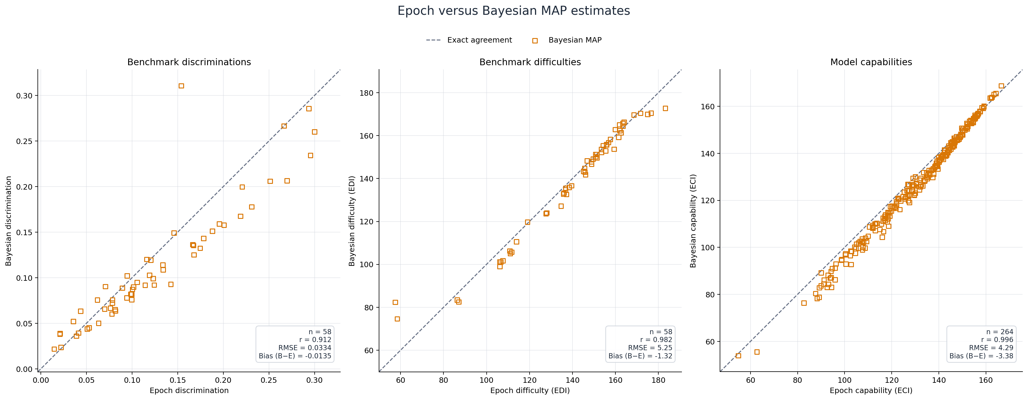
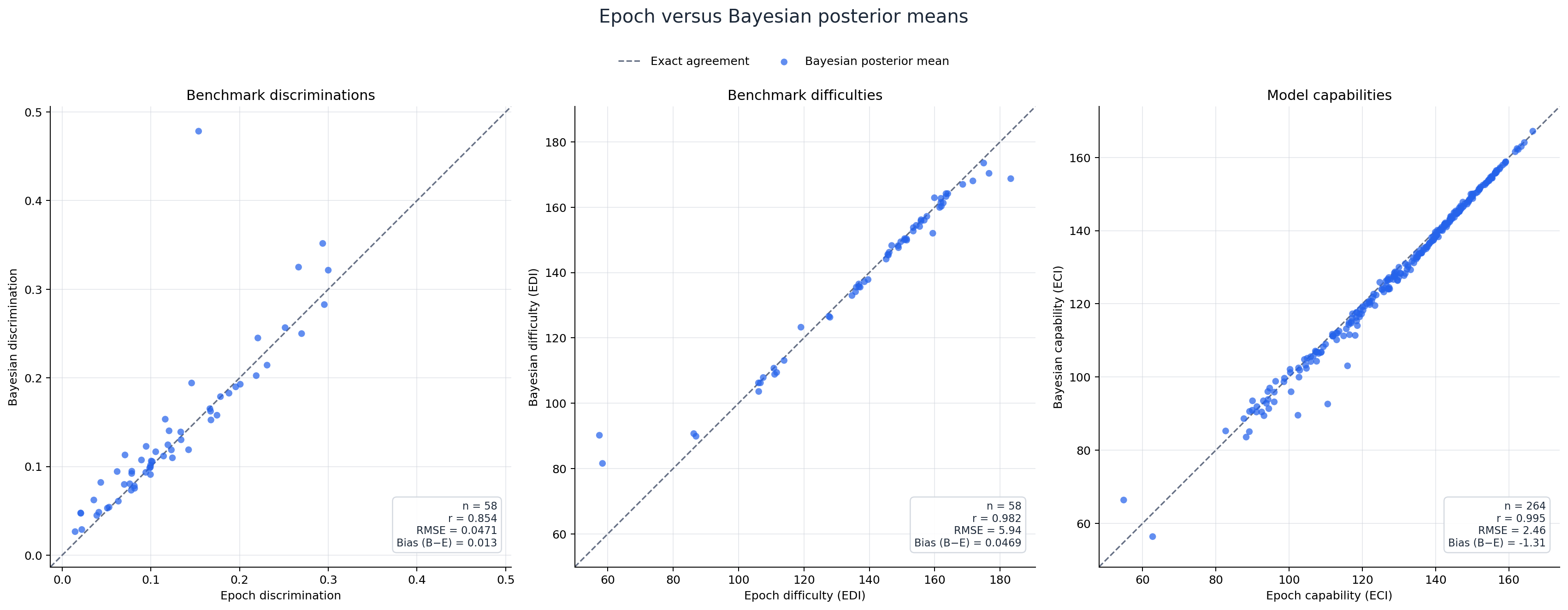
So, should we throw out the ECI because it uses static parameters and try something new? No. It turns out that predicted model capabilities taking changing parameters into account correlate at 0.995 with Epoch’s predicted model capabilities, making them nearly identical. The same holds for benchmark difficulties, which correlate at 0.98, though at the extremes my estimates suggest that the hardest benchmarks aren’t quite as hard as Epoch estimates and the easiest benchmarks aren’t quite as easy. Benchmark discriminations are less correlated, at only 0.85, but there’s no discernible systematic pattern to the differences.
Still, it does mean we need to be careful when treating AI capability as a unitary construct, as the ECI does. Which capabilities are most relevant changes over time, partly because labs shift their focus. It used to be reading and understanding language, but as models became proficient at that, attention shifted toward coding and mathematics. A chart that represents AI progress with a single capability score is therefore somewhat misleading: what counts as capability changes over time. Progress in currently relevant capabilities, such as mathematics and coding, may be underestimated by combining them with benchmarks that emphasize domains in which progress is now slower, such as general language understanding. Those benchmarks pull the construct the ECI is measuring towards slower-moving domains.
In conclusion, the ECI remains a (very) useful summary of average benchmark performance, but it should not be mistaken for a measure of a single, unchanging construct. We should take care to think about which capabilities we think are useful to measure.
Appendix
The Real Treasure Was The Models We Made Along The Way
I didn’t begin with the final two-stage model. I started by reproducing Epoch’s estimator as literally as possible, then changed one assumption at a time, to ensure I wasn’t making any silly mistakes. Expand the steps below to follow the progression from the public ECI implementation to the two-stage model used in this post. (You could always just skip to the final model, but I think it’s easier to go step-by-step.)
The code, frozen data, and compact results for all six models are available in the accompanying GitHub repository.
1. Bayesianizing the ECI
The core of Epoch’s model is, as described above, the logistic function (source) (line 242 of the ECI implementation):
\[\mu_{mb} = \sigma(\alpha_b[C_m-D_b])\]where:
\[\sigma(x) = \frac{1}{1+e^{-x}}\]Free parameter vector
There are $M$ models and $B$ benchmarks. Epoch’s implementation estimates:
\[\phi = (C_1, \dots, C_M,D_1,\dots,D_B,\alpha_1,\dots,\alpha_{B-1})\]There is one benchmark discrimination excluded from the free parameter vector: Winogrande’s discrimination, which is fixed at 1. The number of free parameters is therefore:
\[K = M + 2B - 1\]The raw parameter bounds are (lines 257-266 of the ECI implementation):
\[-10 \leq C_m \leq 10\] \[-10 \leq D_b \leq 10\] \[0.1 \leq \alpha_b \leq 10\]Observed scores are clipped to $[0.001,0.999]$ before fitting (lines 196-197 of the ECI implementation).
Implemented residual vector
For every observed score, the code (line 243 of the ECI implementation) supplies SciPy with its residual:
\[r_{mb}(\phi) = \mu_{mb}(\phi) - s_{mb}\]It also appends a residual used for regularization (lines 245-246 of the ECI implementation):
\[r_\text{reg}(\phi) = \sqrt{\lambda \frac{1}{K} \sum_{k=1}^{K}\phi_k^2}\]where the default regularization strength, $\lambda$ is set to 0.1 (line 138 of the ECI implementation).
Scipy’s least_squares minimizes one-half of the sum of squared residuals, so Epoch’s actual implemented objective is:
Public scale
After fitting, Epoch converts the raw capabilities to the official ECI scale using an affine transformation while setting Claude 3.5 Sonnet at 130 and GPT-5 at 150.
Exact MAP-equivalent model
A model’s performance on a benchmark is modeled as:
\[s_{mb}\mid\phi \sim \mathcal N\left(\mu_{mb}(\phi),\sigma_\varepsilon^2\right).\]where $\sigma_\varepsilon$ is a fixed residual standard deviation.
Ignoring constants, the negative log-likelihood is:
\[-\log p(s\mid\phi) = \frac{1}{2\sigma_\varepsilon^2} \sum_{(m,b)\in\mathcal O} \left[s_{mb}-\mu_{mb}(\phi)\right]^2.\]We place independent Gaussian priors with a common standard deviation $\tau$ on the free parameters, subject to the same bounds used by Epoch:
\[C_m\sim\operatorname{TruncatedNormal}(0,\tau^2;-10,10),\] \[D_b\sim\operatorname{TruncatedNormal}(0,\tau^2;-10,10),\]and:
\[\alpha_b \sim \operatorname{TruncatedNormal}(0,\tau^2;0.1,10)\]for each non-Winogrande benchmark. The Winogrande slope remains fixed:
\[\alpha_{\text{Winogrande}}=1.\]Away from the bounds, the negative log-prior is:
\[-\log p(\phi) = \frac{1}{2\tau^2} \sum_{k=1}^{K}\phi_k^2 +\text{constant}\]So, the negative log-posterior is
\[-\log p(s\mid\phi) - \log p(\phi) = \frac{1}{2\sigma_\varepsilon^2} \sum_{(m,b)\in\mathcal O} \left[s_{mb}-\mu_{mb}(\phi)\right]^2 + \frac{1}{2\tau^2} \sum_{k=1}^{K}\phi_k^2\]If we multiply the negative log-posterior by $\sigma_\epsilon^2$, we get:
\[\frac{1}{2} \sum_{(m,b)\in\mathcal O} \left[s_{mb}-\mu_{mb}(\phi)\right]^2 + \frac{1}{2} \frac{\sigma_\varepsilon^2}{\tau^2} \sum_{k=1}^{K}\phi_k^2\]This matches Epoch’s objective when:
\[\boxed{ \frac{\lambda}{K} = \frac{\sigma_\varepsilon^2}{\tau^2} }\]or equivalently:
\[\boxed{ \tau = \sigma_\varepsilon\sqrt{\frac{K}{\lambda}} }.\]It’s important to note that there’s no unique pair $(\sigma_\epsilon, \tau)$ implied by the objective. Only the ratio is implied. We could set $\sigma_\epsilon = 1$, but, since the scores lie in $[0.001, 0.999]$, a residual standard deviation of 1 would be absurdly large on the observed scale.
What’s more, this also affects $\tau$. For example, if $K = 379$ and $\lambda = 0.1$, then setting $\epsilon_e = 1$ implies
\[\tau = \sqrt{379/0.1} \approx 61.6\]This is nearly flat over the capability and difficulty bounds $[-10, 10]$ and the discrimination bounds $[0.1, 10]$. As such, the penalty isn’t really doing much.
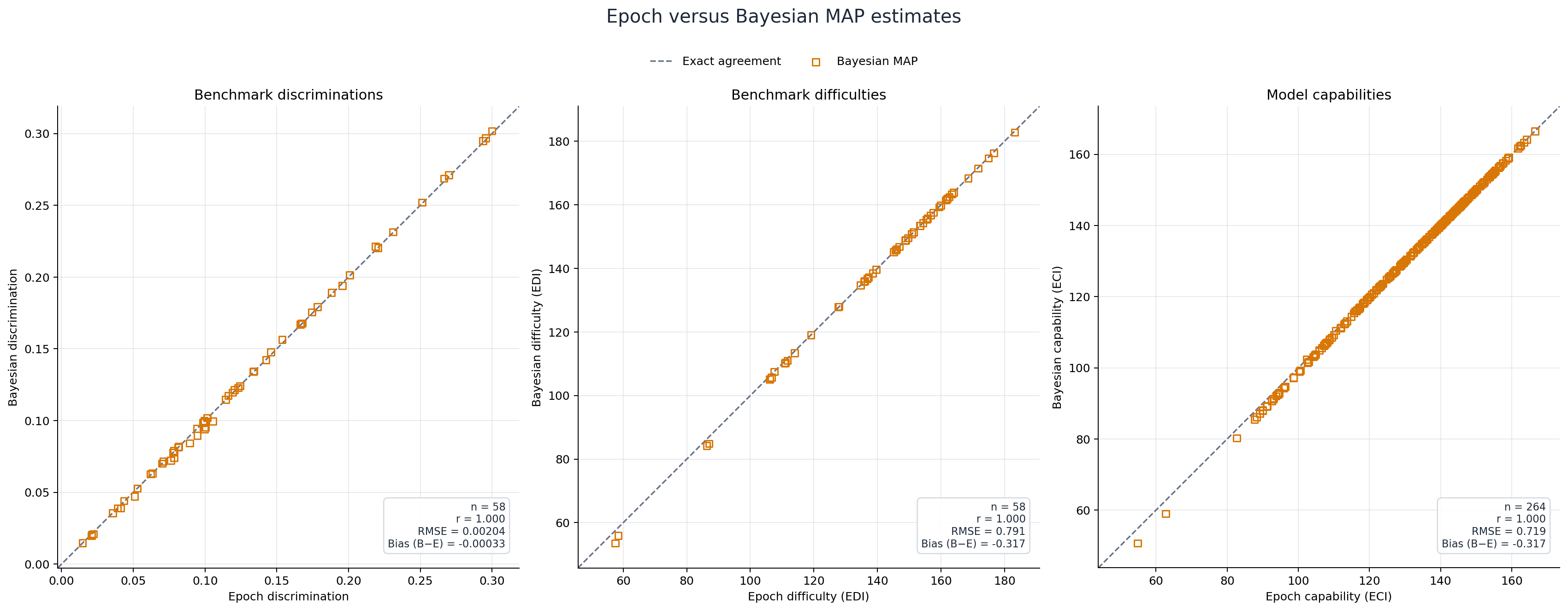
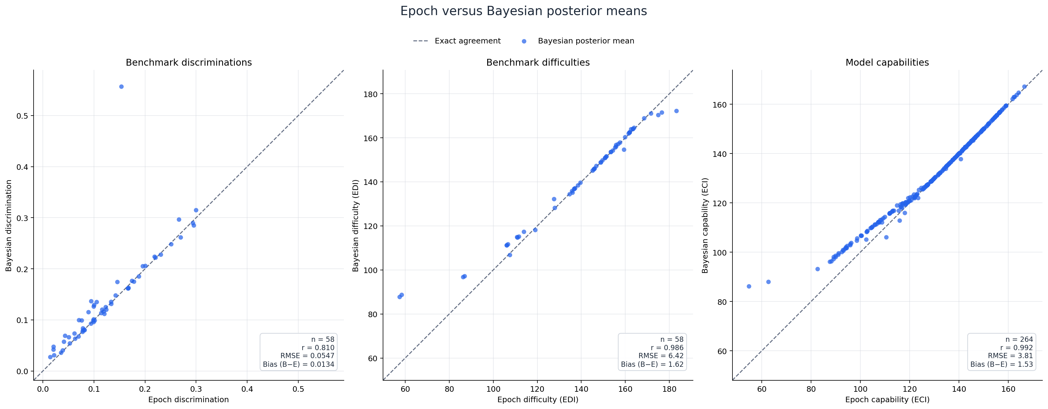
Unfortunately, I first ended up doing taking the ‘convenient’ approach of setting $\sigma_\epsilon = 1$, and so while the MAP estimates match exactly, the posterior means are all over the place.
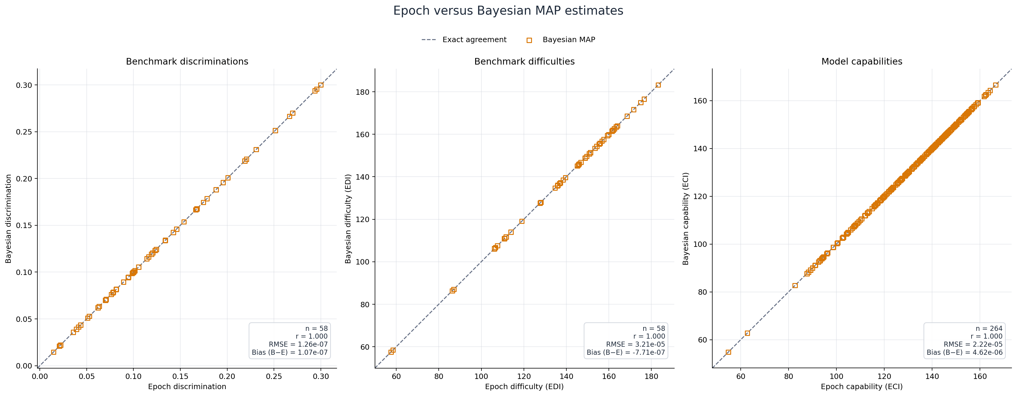
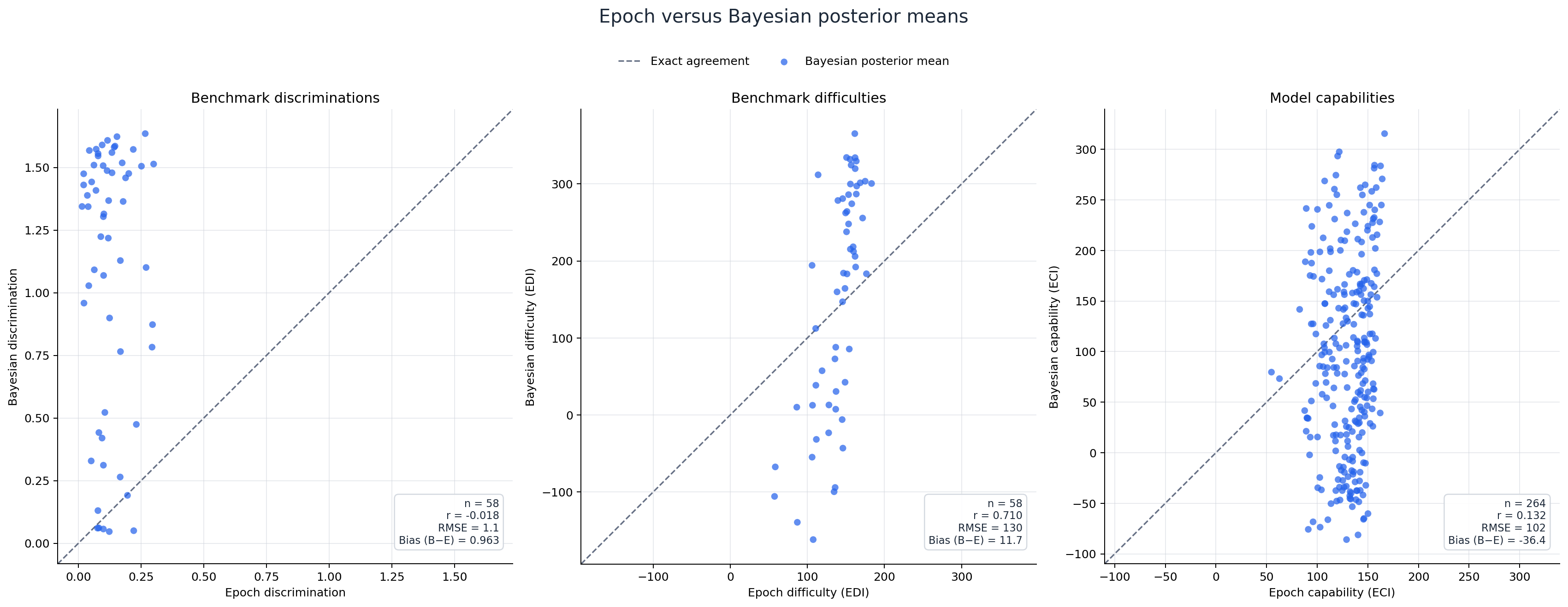
2. Learning the Residual Scale
The first model set $\sigma_\varepsilon$ to 1 because that was convenient. However, a residual standard deviation of 1 is absurdly large for scores bounded between 0 and 1 (well, technically between 0.001 and 0.999). Given that only the ratio $\frac{\sigma_\varepsilon^2}{\tau^2}=\frac{\lambda}{K}$ matters, it might be better to let the model fit the residual standard deviation instead.
So, the second model I fit assigns
\[\log\sigma_\varepsilon\sim\mathcal N(\log 0.1,1)\]and deterministically sets
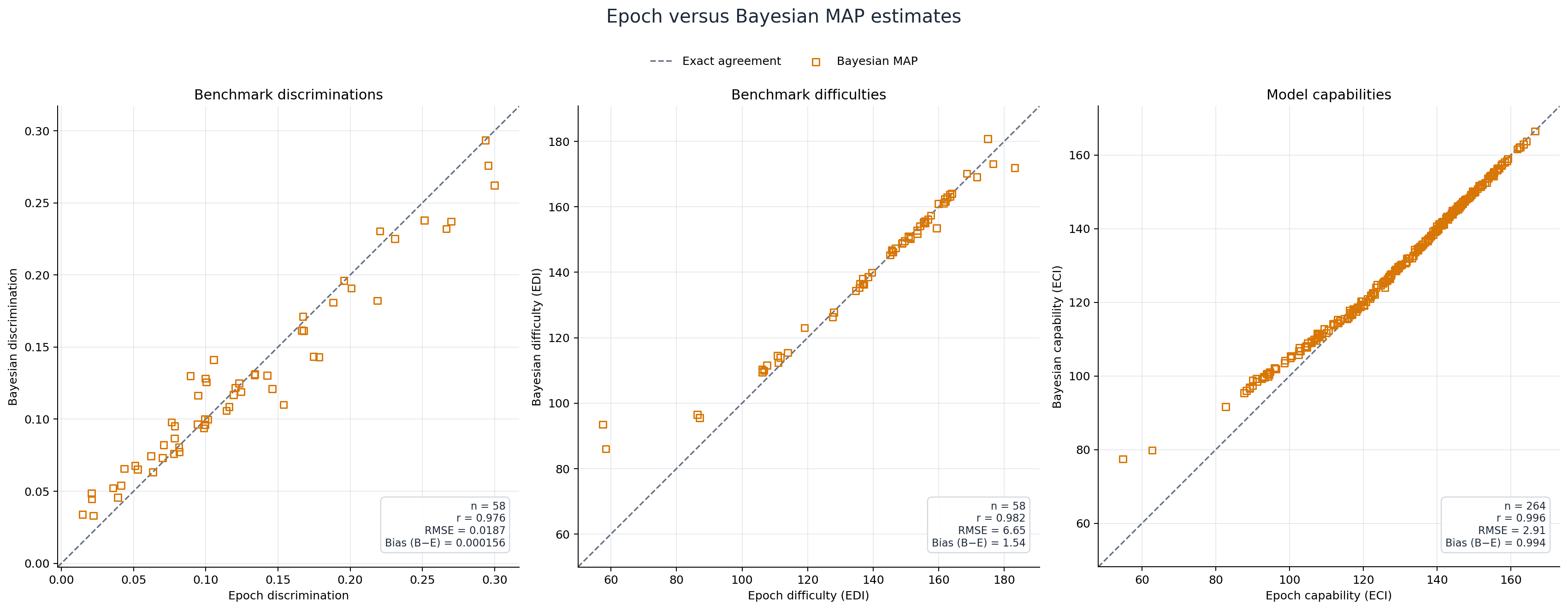
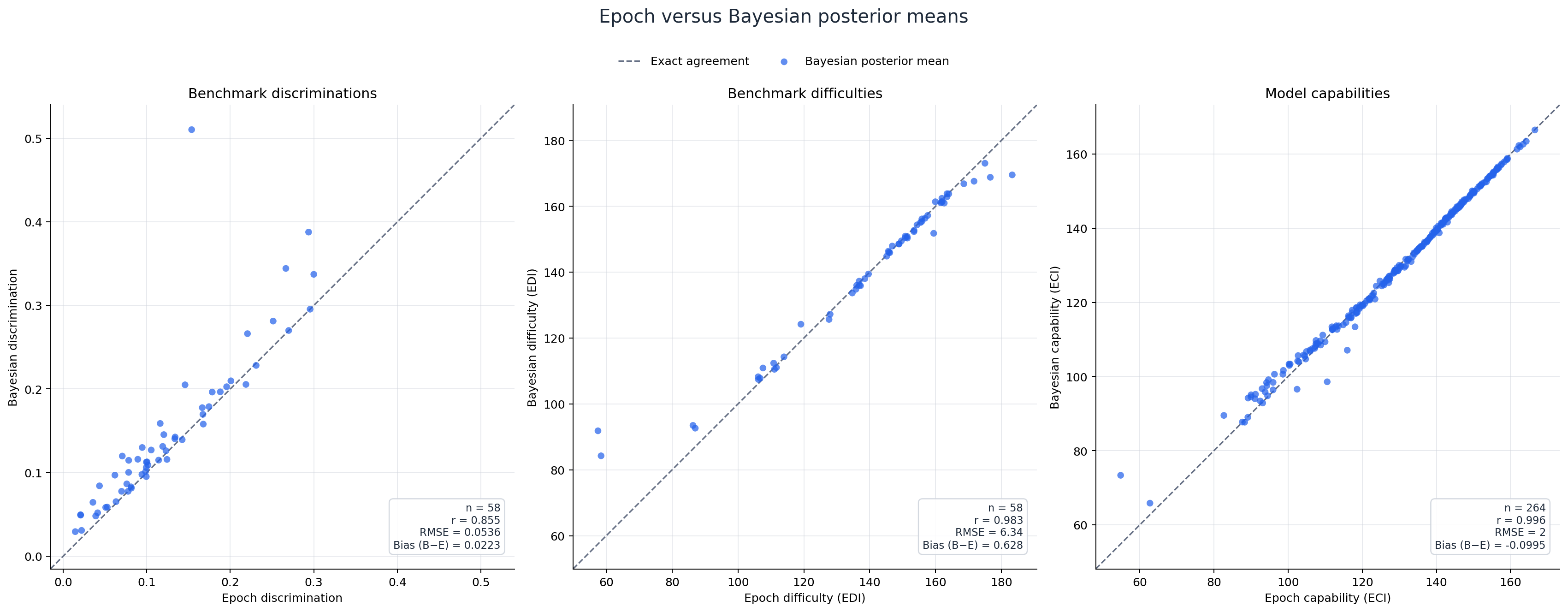
\[\tau=\sigma_\varepsilon\sqrt{\frac{K}{\lambda}}.\]For any value of $\sigma_\varepsilon$, the model has the same variance-to-penalty ratio as Epoch, but now it can learn the appropriate residual variance from the data. Everything else remains unchanged: Winogrande’s discrimination is fixed at 1, capabilities and difficulties remain bounded to $[-10,10]$, and the other discriminations remain bounded to $[0.1,10]$. As you can see, the MAP estimates still match Epoch’s exactly, while the posterior mean estimates are much more reasonable, though there’s a bend in the curve starting below an ECI of ~120 such that the Bayesian estimates are higher than Epoch’s estimates.
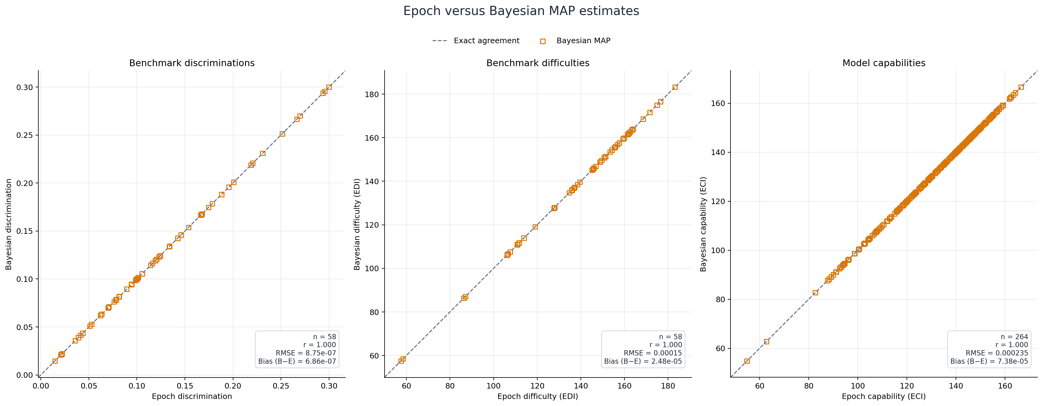
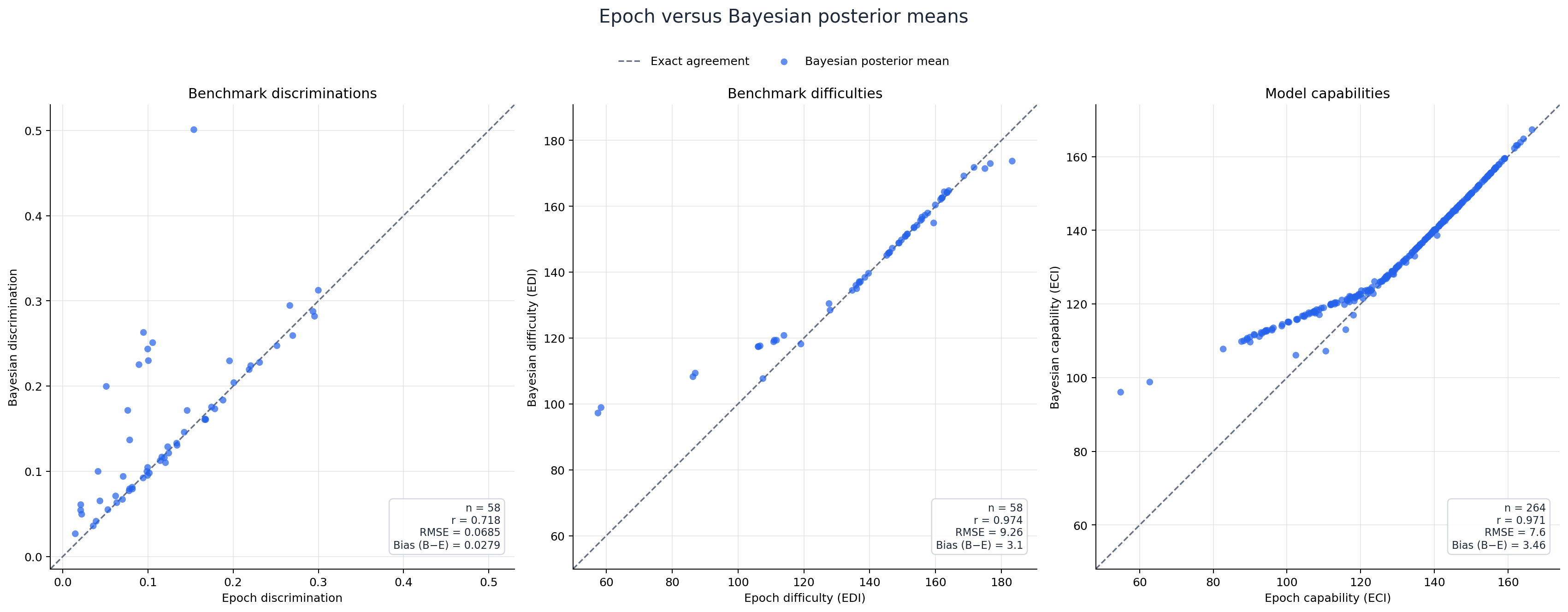
3. Unfixing Winogrande
The next model estimates Winogrande’s discrimination along with every other benchmark discrimination. There are now
\[K=M+2B\]free ECI parameters, and every discrimination receives the same bounded Gaussian prior:
\[\alpha_b\sim\operatorname{TruncatedNormal}(0,\tau^2;0.1,10).\]Removing the Winogrande anchor creates a scale identifiability issue. For any $a>0$,
\[C_m'=aC_m,\qquad D_b'=aD_b,\qquad \alpha_b'=\frac{\alpha_b}{a}\]produces exactly the same predictions. The likelihood is also unchanged when the same constant is added to every capability and difficulty. The bounded proper priors make the posterior proper and select a particular origin and unit, but I still don’t like the model.
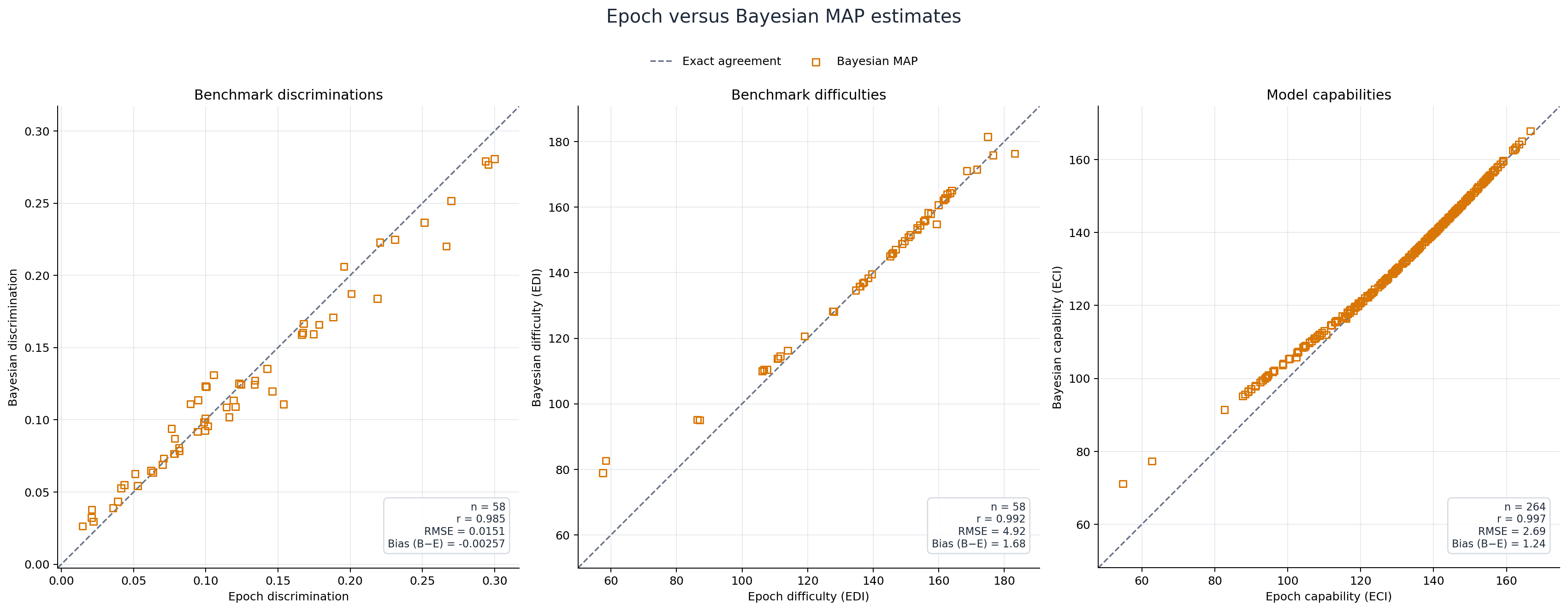
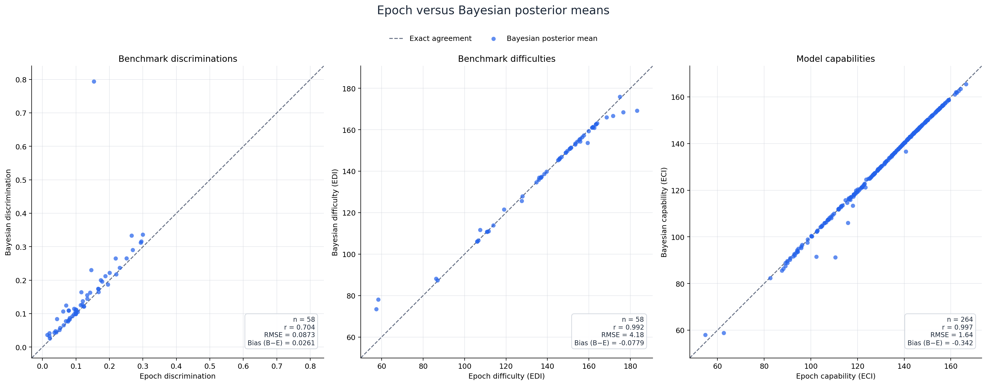
Nevertheless, it’s still a useful intermediate model. If we’re to model changes in discriminations, we can’t also fix the discrimination of one of the benchmarks. The model produces MAP estimates, that no longer exactly match those of Epoch, but are still extremely close. The posterior mean estimates have also gotten closer to Epoch’s estimates.
4. Replacing the Anchor and Bounds with Symmetric Identification
Our next model removes the hard bounds and resolves the identifiability issue without privileging a particular model or benchmark.
Capabilities and difficulties are combined into one vector and assigned a zero-sum Gaussian prior:
\[(C_1,\ldots,C_M,D_1,\ldots,D_B) \sim\operatorname{ZeroSumNormal}(\tau),\]which enforces
\[\sum_m C_m+\sum_bD_b=0.\]This identifies the origin of the latent scale. Discriminations are modeled on a logarithmic scale:
\[s_\alpha\sim\operatorname{HalfNormal}(0.5),\] \[(\log\alpha_1,\ldots,\log\alpha_B) \sim\operatorname{ZeroSumNormal}(s_\alpha).\]Therefore,
\[\sum_b\log\alpha_b=0\]and the geometric mean of the discriminations is one:
\[\left(\prod_b\alpha_b\right)^{1/B}=1.\]This identifies the multiplicative scale. This static model becomes the foundation for the parameter-varying models. Also, our posterior mean estimates are finally lining up with Epoch’s estimates, which is nice.
5. Allowing Discriminations to Change Over Time
The first parameter-varying model keeps capabilities and difficulties static but allows benchmark discriminations to depend on model-release month. Let $t_{0b}$ be benchmark $b$’s earliest observed month. Its initial log discrimination receives the prior described above:
\[s_\alpha\sim\operatorname{HalfNormal}(0.5),\] \[(a_{1,0},\ldots,a_{B,0}) \sim\operatorname{ZeroSumNormal}(s_\alpha).\]Temporal change follows a stationary RBF Gaussian process. All benchmarks share the same length scale,
\[\ell_\alpha\sim\operatorname{Uniform}(2,36),\]which is measured in months. The covariance function is given by
\[K_{\alpha,tt'} = \exp\left[-\frac{(t-t')^2}{2\ell_\alpha^2}\right]+10^{-4}I.\]Each benchmark has its own Gaussian process trajectory $f_b$:
\[f_b\sim\mathcal N(\mathbf 0,K_\alpha),\] \[\kappa_b\sim\operatorname{HalfNormal}(0.5).\]A benchmark’s monthly discrimination is given by
\[\log\alpha_{b,t} = a_{b,0}+\kappa_b\left(f_{b,t}-f_{b,t_{0b}}\right).\]The likelihood for observed scores is
\[s_{mb} \sim \mathcal N\left( \sigma\left[\alpha_{b,t_m}(C_m-D_b)\right], \sigma_\varepsilon^2 \right).\]When a single discrimination is needed for a model (such as in the following graphs), I use the geometric mean across a benchmark’s supported months. This is the first stage of the final analysis.
6. The Final Two-Stage Model
The analysis in this post uses a two-stage model. Stage 1 was the model described I just described above. For Stage 2, rather than passing only Stage 1’s posterior means, I use discrimination draws
\[\boldsymbol\alpha^{(q)} = \{\alpha^{(q)}_{b,t}:b=1,\ldots,B;\ t=1,\ldots,T\}.\]This allows us to use and model the posterior distribution of Stage 1’s results, rather than treating the posterior mean as the only possible set of discriminations.
Each draw is normalized such that its geometric mean of the discriminations is equal to 1. If $\mathcal T_b$ is benchmark $b$’s supported calendar range, define the average log discrimination, $g^{(q)}$ as
\[g^{(q)} = \frac{1}{B} \sum_b \left[ \frac{1}{|\mathcal T_b|} \sum_{t\in\mathcal T_b} \log\alpha^{(q)}_{b,t} \right].\]The draw we end up using is
\[\widetilde\alpha^{(q)}_{b,t} = \exp\left[\log\alpha^{(q)}_{b,t}-g^{(q)}\right].\]This normalization does not alter relative differences between benchmarks or temporal changes within a benchmark; it only fixes the otherwise arbitrary unit of the latent scale.
For every propagated draw, I fit a model in which the difficulties can vary across time. The set of discriminations is fixed within that fit, while capabilities and benchmark difficulties are re-estimated. Difficulty deviations follow another shared-length-scale RBF process:
\[\ell_D\sim\operatorname{Uniform}(2,36),\] \[h_b\sim\mathcal N(\mathbf 0,K_D),\] \[\omega_b\sim\operatorname{HalfNormal}(0.5).\]Let the raw temporal-difficulty be
\[r_{b,t}=\omega_bh_{b,t}.\]The raw temporal-difficulties could absorb both benchmark averages and a movement shared by all benchmarks in a calendar month. To prevent that, we impose the constraint
\[\sum_{t\in\mathcal T_b}\delta_{b,t}=0\]for every benchmark. Thus, the deviations average to zero across each benchmark’s supported months and do not change its overall difficulty. We also impose
\[\sum_{b:(b,t)\text{ supported}}\delta_{b,t}=0\]for every month. Thus, within each month, the deviations average to zero across the benchmarks used in that month. So deviations measure how benchmark difficulties change relative to one another. Monthly difficulty is then
\[D_{b,t}=\bar D_b+\delta_{b,t},\]and the conditional likelihood is
\[s_{mb} \sim \mathcal N\left( \sigma\left[ \widetilde\alpha^{(q)}_{b,t_m} (C_m-D_{b,t_m}) \right], \sigma_\varepsilon^2 \right).\]I repeat this fit for complete surfaces drawn from Stage 1 and pool the conditional posteriors:
\[p_{\mathrm{mod}}(\Theta_D\mid s) \approx \frac{1}{Q} \sum_{q=1}^{Q} p_2\left( \Theta_D\mid s,\widetilde{\boldsymbol\alpha}^{(q)} \right).\]This results in our final estimates, which, when we ignore changes in discriminations and difficulties over time, match Epoch’s estimates pretty well.
-
Marc Brysbaert, Paweł Mandera, Samantha F. McCormick, and Emmanuel Keuleers, “Word Prevalence Norms for 62,000 English Lemmas,” Behavior Research Methods 51 (2019): 467–479, https://doi.org/10.3758/s13428-018-1077-9 ↩